Historical Greeks and Implied Volatility Expand Massive's Options Data
Nov 20, 2026
Massive's options data now includes Historical Greeks & IV, a new endpoint that returns end of day delta, gamma, theta, vega, rho, and implied volatility for every listed U.S. options contract on every trading day. Each row also carries the inputs used to compute those values, including the option's bid, ask, and midpoint, the underlying price, the risk free rate, the dividend yield, and the timestamps of the quotes behind them, so you can see exactly how each number was produced. Building this yourself used to mean collecting synchronized quotes for both the option and the underlying, a Treasury curve, and dividend history, then running a pricing model across millions of contracts. Now one request returns a full option chain for any day back to September 1, 2022. Historical Greeks & IV is included in the Options Advanced plan and the Historical Options Analytics Business plan.
What Historical Greeks Are
The Greeks describe how an option's price responds to the inputs that drive it: delta to the underlying price, gamma to changes in delta, theta to time, vega to implied volatility, and rho to interest rates. Implied volatility is the volatility that makes a pricing model match the option's market price, and it is the standard way to compare how expensive options are.
None of these values can be read from the market. Producing them for a past date takes option and underlying prices sampled at the same moment, rates, dividends, and a model that handles early exercise, run across roughly a million contracts per day and terabytes of quote history. Few teams can justify building that, which is why historical Greeks have been one of the most requested additions to our options data.
Most of those requests come down to testing ideas against the past. Many options strategies are defined by delta or implied volatility rather than price, such as selling the 16 delta put 45 days out, so a backtest has to know what those values were on each day. Volatility traders need a long history to judge whether implied volatility is high or low today, which is what measures like IV rank are built on, and earnings traders want to compare the move the market priced before each report with the move that followed. Researchers use skew and the volatility term structure as signals, risk teams break P&L into its Greeks and run historical stress tests, and companies building trading tools need the same history to show their own users.
Each row is taken from one fixed snapshot 15 minutes before the close, priced with the same model, and returned with every input, so values stay consistent from day to day. It uses the same option tickers as our trades, quotes, open interest, and aggregates endpoints, so the rest of a contract's data is one call away. The examples below use the Massive Python client.
Historical Greeks & IV API
The Historical Greeks & IV endpoint returns one row per contract per trading day. You can filter by a single contract with ticker, by an entire chain with underlying_ticker, and narrow further with expiration_date, contract_type, and a date or date range.
Here is how to look up one NVIDIA contract on November 18, 2026.
Request Example
from massive import RESTClient

client = RESTClient("YOUR_API_KEY")

greeks = []
for g in client.list_options_analytics(
    ticker="O:NVDA270115C00170000",
    date="2026-11-18",
):
    greeks.append(g)
print(greeks)
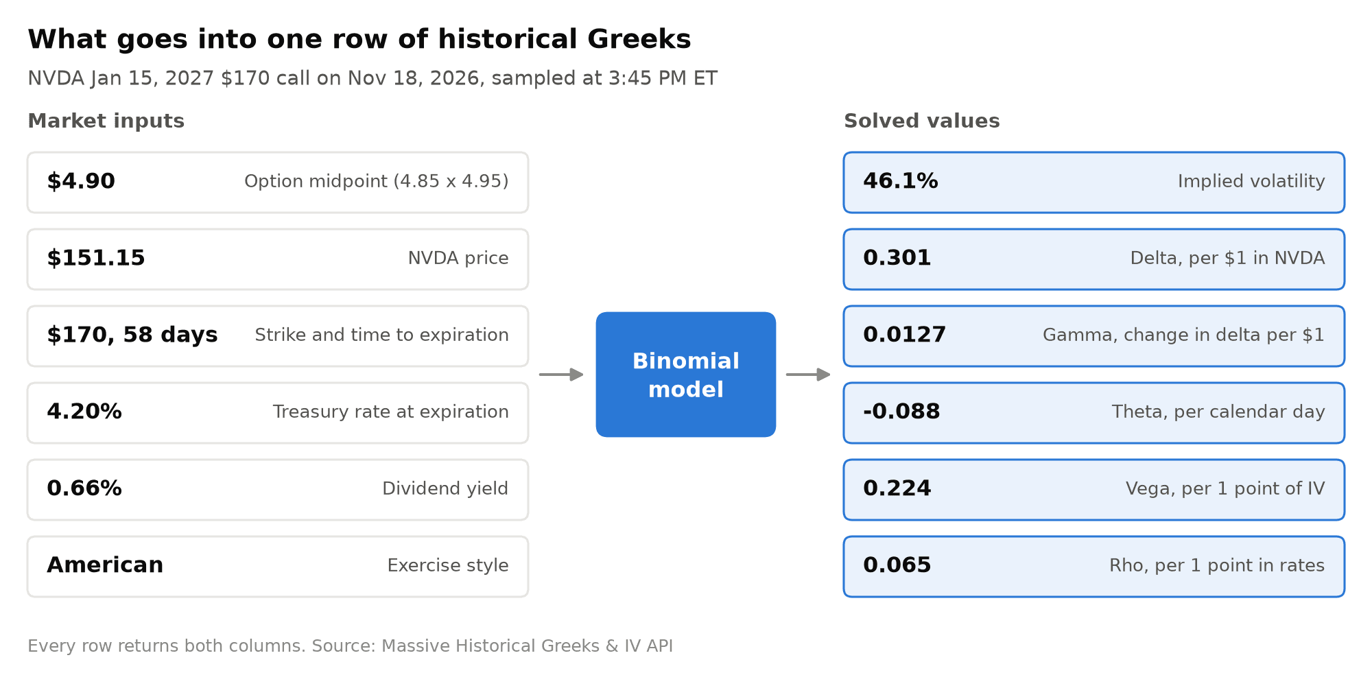
option_price is the midpoint of the national best bid and offer at 3:45 PM ET, or 12:45 PM ET on early close days. The bid, ask, and quote_timestamp fields show the exact quote it came from, and underlying_price is the last trade in the underlying at or before the same moment.
implied_volatility is annualized and expressed as a decimal, so 0.461 means 46.1%. It is solved against option_price with a binomial model, which handles the early exercise feature of American style equity options. The exercise_style field tells you which style each contract uses.
theta, vega, and rho use trader conventions. Theta is the change in price per calendar day, vega is the change for a one point move in implied volatility, and rho is the change for a one percentage point move in rates. All of them are quoted per share, like the option price.
risk_free_rate is the Treasury yield interpolated to the option's expiration, and dividend_yield annualizes the most recent regular dividend. Both are decimals, and having them in each row means you can reproduce a value or reprice the contract under your own assumptions.
open_interest is the figure published on the morning of date for the prior session, and volume is the number of contracts traded on date.
Some rows come back with null Greeks. This happens when a contract has no quote at the snapshot or when its midpoint is below the option's intrinsic value, which is common for deep in the money contracts with wide markets. Those rows still include the bid, ask, and underlying price, so you can see why no value was solved. On November 18, 962 of the 4,190 NVDA contracts were in this state.
Leaving out ticker and passing underlying_ticker with a date returns the full chain for that day. That is the request most of the demo below is built on, and for NVDA it returned all 4,190 contracts in a single page in under a second.
Demo: NVIDIA's Q3 Earnings Through the Greeks
Earnings reports are a good test for historical Greeks because they produce some of the largest and most predictable changes in implied volatility. NVIDIA reported its fiscal third quarter after the close on November 17, 2026. We will use the chains from the sessions before and after that report to see how much movement the options market expected, how volatility changed once the news was out, and what that meant for one contract.
The first step is a helper that takes one day's chain and finds the at the money implied volatility for each expiration. It uses the strike nearest the underlying price, averages the call and put implied volatility at that strike, and also keeps the price of the straddle, which is the call plus the put.
from collections import defaultdict
from massive import RESTClient
client = RESTClient("YOUR_API_KEY") # pagination on: iterates every pagedefchain(day):returnlist(client.list_options_analytics(
underlying_ticker="NVDA", date=day, limit=50000))
defatm_iv(rows):"""At-the-money IV and straddle price for each expiration in one day's chain.""" spot = next(r.underlying_price for r in rows if r.underlying_price)
pairs = defaultdict(dict)
for r in rows:
if r.implied_volatility isnotNone:
pairs[(r.expiration_date, r.strike_price)][r.contract_type] = r
out = {}
for exp insorted({e for e, _ in pairs}):
strikes = [k for k in pairs if k[0] == exp andlen(pairs[k]) == 2]
ifnot strikes:
continue k = min(strikes, key=lambda k: abs(k[1] - spot))
call, put = pairs[k]["call"], pairs[k]["put"]
out[exp] = {
"spot": spot,
"strike": k[1],
"iv": (call.implied_volatility + put.implied_volatility) / 2,
"straddle": call.option_price + put.option_price,
}
return out
before, after = atm_iv(chain("2026-11-17")), atm_iv(chain("2026-11-18"))
print(f"{'Expiration':<12}{'Nov 17':>9}{'Nov 18':>9}{'Change':>9}")
for exp in ["2026-11-20", "2026-11-27", "2026-12-18", "2027-01-15", "2027-03-19", "2027-06-17"]:
b, a = before[exp]["iv"], after[exp]["iv"]
print(f"{exp:<12}{b:>9.1%}{a:>9.1%}{(a - b) * 100:>+9.1f}")
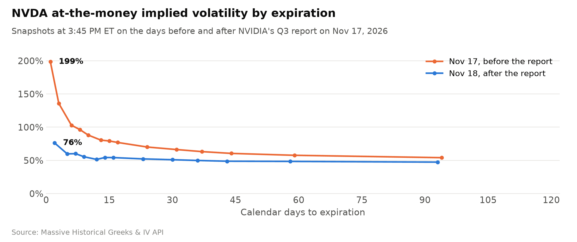
Before the report, the options expiring that Friday were priced at 135.8% implied volatility, and the contracts expiring the next day were priced at 199%. One session later the Friday options had dropped to 76.3%. The drop gets smaller further out because the report is one day out of many in a longer dated option's life, so removing it changes the average volatility over that life much less. This pattern is usually called a volatility crush, and plotting both days by days to expiration shows it clearly.
The price of the at the money straddle in the first expiration after a report is a common rough estimate of how far the market expects the stock to move. Massive's Benzinga Earnings endpoint provides the report dates, and the daily Aggregates endpoint provides the actual moves, so we can compare the two for NVIDIA's last five reports. The earnings data is part of our Benzinga partner data and requires a Benzinga plan. If you do not have one, you can replace the reports list with your own report dates and the rest of the code works the same way.
from datetime import UTC, datetime
reports = sorted(
e.date for e in client.list_benzinga_earnings(
ticker="NVDA", date_gte="2025-11-01", date_lte="2026-11-18")
if e.date_status == "confirmed")
closes = {
datetime.fromtimestamp(a.timestamp / 1000, UTC).date().isoformat(): a.close
for a in client.list_aggs("NVDA", 1, "day", "2025-11-01", "2026-11-18")
}
days = sorted(closes)
print(f"{'Report':<12}{'Expiration':<12}{'Straddle':>10}{'Implied':>9}{'Actual':>9}")
for d in reports:
atm = atm_iv(chain(d))
exp = min(e for e in atm if e > d) # first expiration after the report implied = atm[exp]["straddle"] / atm[exp]["spot"]
actual = closes[days[days.index(d) + 1]] / closes[d] - 1print(f"{d:<12}{exp:<12}{atm[exp]['straddle']:>10.2f}{implied:>9.1%}{actual:>+9.1%}")
The market priced a larger move into this report than any of the previous four, about 8.4% using the contracts that expired the next day. NVDA closed 2.9% lower. In four of the five reports the stock moved less than the straddle implied, and the one exception was August 2026, when it rose 8.7% against an implied 5.9%. Five reports are far too few to draw conclusions from, but the same loop runs over any underlying with earnings data, and the history goes back to 2022.
A single day's chain shows the term structure at one point in time. Pulling one chain per session shows how volatility moved over a longer period. The function below interpolates the at the money volatility of the expirations on either side of 30 days to get a constant 30 day measure. Volatility indexes like the VIX also report a constant 30 day value, although they are built from a much wider range of strikes. A thread pool fetches a full year of NVDA chains in parallel:
import math
from concurrent.futures import ThreadPoolExecutor
from datetime import date
defiv30(day, atm):"""Interpolate total variance between the expirations on either side of 30 days.""" d0 = date.fromisoformat(day)
pts = [((date.fromisoformat(e) - d0).days, v["iv"]) for e, v in atm.items()]
lo = max(p for p in pts if0 < p[0] <= 30)
hi = min(p for p in pts if p[0] >= 30)
if lo[0] == hi[0]:
return lo[1]
w_lo, w_hi = lo[1] ** 2 * lo[0], hi[1] ** 2 * hi[0]
w = w_lo + (w_hi - w_lo) * (30 - lo[0]) / (hi[0] - lo[0])
return math.sqrt(w / 30)
sessions = [d for d in days if d >= "2025-11-17"]
with ThreadPoolExecutor(8) as pool:
chains = dict(zip(sessions, pool.map(chain, sessions)))
implied = {d: iv30(d, atm_iv(rows)) for d, rows in chains.items()}
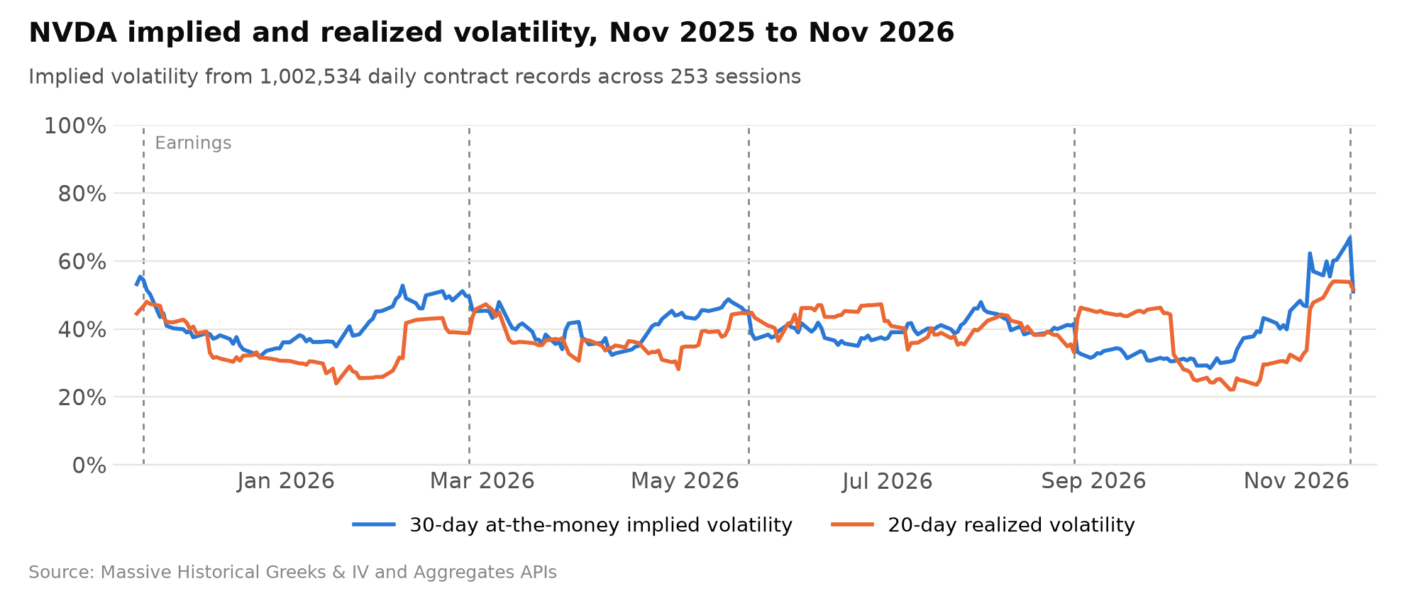
That is 1,002,534 contract records across 253 sessions, and it took about 28 seconds to download. The chart compares the result with NVDA's 20 day realized volatility, calculated from the same daily closes.
The 30 day implied volatility built up ahead of each report and fell the next day, by 3 to 16 points. The most recent run up was the largest of the year, from a low of 28.5% on October 6 to 66.8% the afternoon before the report, during a period when NVDA fell from $173.73 to $155.46 in four sessions. Over the full year, implied volatility averaged 40.4% and realized volatility averaged 37.6%, and implied was higher on 66% of days. The difference between implied and realized volatility is how researchers study the volatility risk premium, and having both historical series in one place makes it easier to analyze how that relationship changes over time and across underlyings.
Last, the Greeks in each row explain why an individual contract's price changed. The NVDA January 2027 $170 call fell from $8.15 to $4.90 between the two snapshots. Using the Greeks from November 17 and the change in the underlying and implied volatility, we can split that loss into its parts:
pre, post = client.list_options_analytics(
ticker="O:NVDA270115C00170000",
date_gte="2026-11-17",
date_lte="2026-11-18",
sort="date.asc",
)
d_spot = post.underlying_price - pre.underlying_price
d_vol = (post.implied_volatility - pre.implied_volatility) * 100# in vol points
parts = {
"Delta": pre.delta * d_spot,
"Gamma": 0.5 * pre.gamma * d_spot ** 2,
"Vega": pre.vega * d_vol,
"Theta": pre.theta * 1, # one calendar day}
print(f"Underlying {pre.underlying_price:.2f} -> {post.underlying_price:.2f}, "f"IV {pre.implied_volatility:.1%} -> {post.implied_volatility:.1%}")
for name, value in parts.items():
print(f"{name:<10}{value:>+8.2f}")
print(f"{'Estimate':<10}{sum(parts.values()):>+8.2f}")
print(f"{'Actual':<10}{post.option_price - pre.option_price:>+8.2f}")
Underlying 153.82 -> 151.15, IV 56.1% -> 46.1%
Delta        -1.01
Gamma        +0.04
Vega         -2.25
Theta        -0.12
Estimate     -3.34
Actual       -3.25
The stock only fell $2.67 between snapshots, which accounts for about a dollar of the loss. Most of the drop came from the 10 point fall in implied volatility, which the vega estimate puts at about $2.25 per share, or $225 per contract. The four terms add up to within 9 cents of the actual change. Three endpoints and about a hundred lines of Python took us from a million rows of Greeks to the expected move, the volatility crush, a year of implied versus realized volatility, and an explanation of one contract's price change.
There are several natural ways to extend this:
You can compare implied volatility across strikes within one expiration to track skew, for example the 25 delta put minus the 25 delta call, and see how it shifts around events.
You can multiply gamma by open_interest across a chain to estimate where gamma is concentrated by strike on any past date.
You can backtest options strategies using point in time Greeks calculated from historical market data with consistent model assumptions, rather than values recomputed with today's inputs.
You can use risk_free_rate, dividend_yield, and option_price to validate your own pricing model against ours, contract by contract.
Next Steps
Historical Greeks & IV is available now in the Options Advanced plan and the Historical Options Analytics Business plan, with end of day data for every listed U.S. options contract and history back to September 1, 2022. Each row includes delta, gamma, theta, vega, rho, and implied volatility, along with the quotes, rates, and dividends used to produce them. It shares tickers with the Trades, Quotes, Open Interest, and Aggregates endpoints we already offer, so the market data around any value is a few calls away. The earnings dates in the demo came from our Benzinga Earnings endpoint, which is available with a Benzinga plan.
If you already use Massive for options data, historical Greeks are now one more piece you can build on, whether you are backtesting a volatility strategy, building surfaces for research, or checking how a position's risk changed over time. You can get started with the Python client and an API key from your dashboard, and our sales team at sales@massive.com can help with business plans and larger integrations.
Disclaimer
This content is for educational purposes only. It is not investment advice or a recommendation to buy or sell any security, and the companies mentioned are used only to illustrate the data.
Massive now offers Historical Greeks & IV, which gives you end-of-day delta, gamma, theta, vega, rho, and implied volatility for every listed U.S. options contract, along with the market inputs behind each value, back to September 2022.
Massive's new Insider Holdings and Insider Activity endpoints turn SEC Form 3, 4, and 5 filings into each insider's current stake and each company's daily net insider buying and selling, so you can screen every U.S. company for insider activity with a single API call.